ENIACU. S. Army
ENIAC
The History of Computing at BRL
A transcript of the BRL story, as told by Mike Muuss on September 25, 1992 to the current laboratory staff and many distinguished former employees and retirees, on the occasion of "Vulnerability Day". This was a part of the celebration commemorating the incorporation of the Ballistic Research Lab (BRL), home of the ENIAC, into the new Army Research Laboratory (ARL).
This document is still being converted from an oral presentation to something really worth reading. Please forgive the rough edges.---DRAFT---
In particular, all the Figures have yet to be scanned in. This is a rather serious deficiency.
There is additional information in my History of Computing Information page.
The history of computing at BRL is inextricably linked with the history of vulnerability/lethality and survivability assessments here at BRL. What I am going to do in this talk is give you a very quick dance through some of the hardware, some of the software, and some of the networking techniques that we have developed. Many of these things were done first here at BRL.
I am going to start by telling you a little bit about the early years when I wasn't here -- my arrival matched up with the advent of mini-computers becoming popular in the labs. I'll tell you in somewhat more detail about that and then end with just a brief taste of what all this technology is good for.
The story begins back in 1935 with a mechanical computer called the Bush Differential Analyzer which showed up here at BRL and it moves forward from there. The proposal for the ENIAC was put together in 1943 and as the ENIAC development proceeded plans for the ORDVAC and EDVAC also came together. Pennsylvania did ENIAC and the Edvac and the University of Illinois contributed on the ORDVAC.
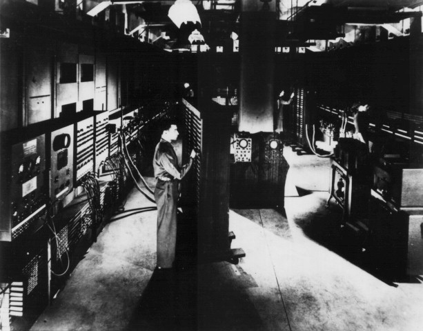 Here is the now classic picture
of the ENIAC
as it was installed at the Moore School of Engineering, University
of
Pennsylvania, with a soldier loading some parameters in. You can
tell it is not
at BRL because the ENIAC was in building 328, and we don't have ceilings
like
that.
Here is the now classic picture
of the ENIAC
as it was installed at the Moore School of Engineering, University
of
Pennsylvania, with a soldier loading some parameters in. You can
tell it is not
at BRL because the ENIAC was in building 328, and we don't have ceilings
like
that.
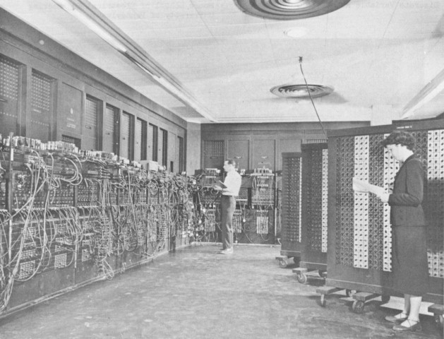 Here is a photo of the ENIAC located in the upper floor
of building 328, at Aberdeen Proving Ground.
Even after the newer machines ORDVAC and EDVAC showed up, the
ENIAC kept being upgraded.
In 1953, it got a gigantic 1,000
words of
memory added to it. Down here in 1956, ORDVAC got an astonishing
4,000
words of memory.
Here is a photo of the ENIAC located in the upper floor
of building 328, at Aberdeen Proving Ground.
Even after the newer machines ORDVAC and EDVAC showed up, the
ENIAC kept being upgraded.
In 1953, it got a gigantic 1,000
words of
memory added to it. Down here in 1956, ORDVAC got an astonishing
4,000
words of memory.
In 1962, when the BRLESC-I went operational at BRL, it was the fastest computer in the world, continuing the tradition started by ENIAC, ORDVAC, and EDVAC. It lost out to the IBM stretch almost immediately, but there weren't very many of those.
Around 1978, BRL got out of the computer-making business and went commercial for it's big machines, and there followed a period of doing things with traditional machines, commercially made machines. I will tell you a little bit more about what happened there in the second part of the talk.
The ENIAC was a decimal machine operating internally on base ten only, using pulse trends to transmit information around. So, to send a nine from one bank of circuits to another bank of circuits, the ENIAC would send nine pulses down the wire, all synchronized by a master clock. This machine sped along at a gargantuan 5,000 operations a second in fixed point only. It is roughly comparable to an HP45 calculator that many of you may have had on your desks when you were working here. Internally, it stored 20 ten-digit numbers, all operating in base ten, and there was no central memory at all. When the machine was originally designed, it was actually a data-flow computer. Numbers moved through the machine along the wiring banks from calculation point to calculation point.
It was John Von Neumann who proposed changing that around and storing the program on two columns of dials in the parameter tables. In the process, this managed to slow the machine down tremendously -- he had created the first Von Neumann bottleneck! I understand he was quite unpopular over at Launch and Flight Division for making their ballistic programs go so much slower. The big advantage to this change was that it was much quicker then to program the machine because you just dialed your program in, rather than having to get an engineer to wire the program for you.
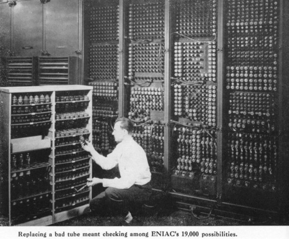 The ENIAC was a
gargantuan beast made from over 19,000 vacuum tubes. Here you can see
some
poor technician of the day trying to figure out which one to replace
-- a job I
don't envy him at all. To interface to the IBM card punch equipment took
15,000
relays because IBM used high current circuits to run all their accounting
machines, and the vacuum tubes could not sink enough current in order
to please IBM.
The ENIAC was a
gargantuan beast made from over 19,000 vacuum tubes. Here you can see
some
poor technician of the day trying to figure out which one to replace
-- a job I
don't envy him at all. To interface to the IBM card punch equipment took
15,000
relays because IBM used high current circuits to run all their accounting
machines, and the vacuum tubes could not sink enough current in order
to please IBM.
ENIAC used 175 kilowatts of power, and it lasted about 5.6 hours, according to the historical reports, between repairs. This is an interesting thread, there have been periods of time when we have enjoyed very reliable computers and periods when we didn't. It is fun to watch the reliability figures bounce back and forth.
The next machine which showed up here at BRL not long after the ENIAC was the EDVAC. Because of a change in the number coding system, this machine achieved a tremendous decrease in size, dropping from 19,000 to 5,000 tubes Instead of sending decimal around internally as pulse trains, it was built using Binary Coded Decimal (BCD). This was the first time BCD was ever used inside a computer.
EDVAC had both fixed and floating point which is another major innovation. Already for the second computer on the planet, we have floating point hardware in the machine. I might also add, the ENIAC had hardware divide and hardware square root, which are things you still rarely find built into CPUs today.
The EDVAC CPU had four registers and a 44-bit word, in keeping with BCD coding system and the ten decimal digits of significance. It had mercury delay lines for memory. According to the history books, there was no problem with vibration from the firing range at the main front, but they had a tremendous problem with thermal stability. They eventually had to put it into an elaborate oven with all sorts of thermostats and thermal buffers. They made it work, but heat and not vibration turned out to be the challenge in making this machine go.
Interestingly enough, this -- the second machine on the planet -- had a tape drive that ran at 75 inches per second. Many computers we buy today have tape drives that are not even this fast. It is fun to watch how storage technology goes faster, then slower, then faster again. EDVAC lasted about eight hours between repairs.

The machine after EDVAC, this time coming from Illinois, was the ORDVAC. They were thoughtful enough to put the name of it on top so I don't get the picture mixed up. This one here has another main major change in the way it was built. This one is a pure binary machine using two's complement fixed point. This machine here, the third machine at BRL and about the fourth or fifth machine around in the world, set the pace for all the computers we know today. Two's complement binary mathematics is how all the machines from IBM PCs to the Cray-II operate.
This machine is getting pretty speedy, it can do 71,000 additions per second. A little bit more than 1,000 multiplications per second. It had three registers and a 15 microsecond core memory. This is a prototype, a forerunner of all the machines that are going to follow for decades after.
This was the first computer that had a real compiler on it. No longer did you have to write machines codes every time you wanted to get something done. The BRL folks thought up this language called FORAST and built a compiler. So now the programmers could write much higher level instructions and let the machines do the translation to machine code. There was a time in the early 1950s where BRL employees were worrying about portable software. When almost nobody else even had computers, we had people here worrying about how to make programs work on different kinds of computers. The FORAST language worked both on the BRLESC and on the ORDVAC, and people ported software back and forth very happily. This has been a theme that has continued for a long time.
In the ORDVAC, the tube counts have gone way down, only 3,000, and the number of transistors is coming up. By today's microprocessing standards, this isn't very many parts -- we have half a million or a million transistors on a single integrated circuit in a package only an inch or two long. Building a computer out of basically 5,000 parts, 5,000 transistor-like parts, is really unthinkable. Considering that there were not very many gates inside this machine, they got a lot of performance out of it!
The next one along was BRLESC-I, and it looked like this. Something to make any science-fiction buff drool a little bit. This is a marvelous display panel. You can see what is happening anywhere inside the machine. As an engineer, I really appreciate things like that!
This system was built entirely by BRL engineers from some standard parts that were developed at the National Bureau of Standards (NBS, now NIST). Originally it was going to be a joint project all the way, but NBS wound up contributing just the submodules, and BRL designed and built those into a real working computer. This is getting pretty fast, this is a fifth of a million instructions per second now, really getting up there. It retains the pure binary two's-complement notion, has a reasonable amount of memory, has a drum on it, and, in order to get to speed, the parts count started creeping back up a little bit, but they still managed to get it into a fairly small package there.
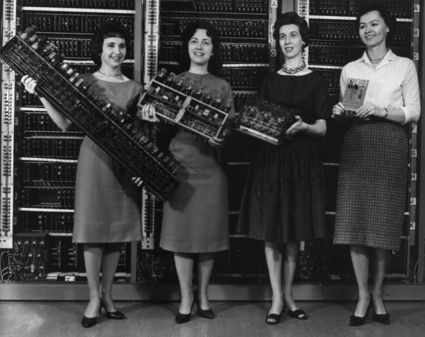
Army photographers took this photo in 1962 to show a comparison between the different technologies used in the first four computers. From left to right, these boards are out the ENIAC, Edvac, ORDVAC, and BRLESC-I. To the best of my understanding, these are roughly comparable circuits. You can see how technology allowed the machines to get smaller. As you make the machines smaller, then you can make them go faster.
The next step really came about for mini computers. Industry was going along the same projection I showed there with parts getting smaller and smaller, and at some point hardware started getting very cheap. So much so that an average Lab Division or department of a University could manage to afford a little computer of their own. Something like a PDP-8 or a PDP-11/20 or eventually, for us, a PDP-11/70. Minicomputers were a lot easier to program than the big machines of the day, and that meant there were a lot more people who wanted to use them. This pushed computing power more and more out to the masses. At this point, technology splits into three main tracks: workstations, mini computers or departmental machines, and super computers.
Our goal in 1980, which we articulated in the ARRADCOM blueprint for the 1980s, was that everybody should have a desk, a chair, a telephone, a computer terminal (which is all we were looking for at the time), a tenth of a million instructions per second per employee (which is basically to say a personal BRLESC-1 for everybody here), and ten megabytes of disk storage. We thought that if we got through this by 1989, if we got this to everybody by 1989, we would be doing very well. In VLD, we actually hit this goal around 1986. That was mostly thanks to aggressive purchasing on the part of Paul Deitz. Here is a picture of kind of where it starts. I'll give you a table and briefly run through some of the developments here.
Background: In 1976 we had remote job entry and some teletype ASR33 type machines with the yellow paper and the punched paper tape -- many of you probably remember them. Special purpose mini computers for laboratory data acquisition, the NOVA, the PDP-8s, we found out in some of the ranges where people had just built a brand new facility and were doing some really good data acquisition. The super computers of the day were the BRLESC-II and some of the analog hybrid machines that Bill Barkuloo had salted away in the basement of building 394 and other places.
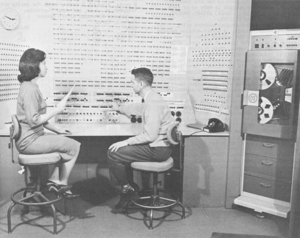
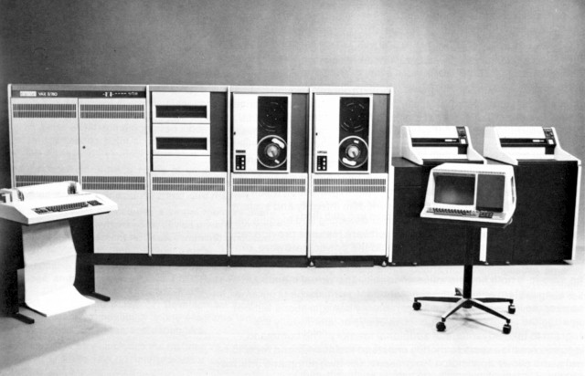
In 1978, we finally started to see ASCII, cathode tube terminals, terminals we all are familiar with now. Harry Reed went out and boldly bought a PDP-11/70 from Digital Equipment Corporation (DEC), and that is the machine you see in the background with the black cabinets and the purple and red controls on the front.
My first visit ever to BRL was in May of 1978, when I was invited by Dr. Steve Wolff (now of NSFNET fame) to give a talk about UNIX, and incidentally, write a driver for an incompatible disk controller that procurement had stuck him with, and install a working system on the new machine.
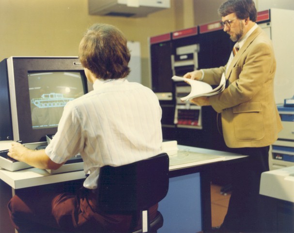
This picture was taken in 1980, and already I was working on applications of interactive graphics. There is the (then) XM1 tank design on the Vector-General "3D" display. I'm sitting there operating it. Next to me, Earl Weaver is consulting a print out of the COMGEOM description representing that XM1 design. I might add, the target description is much thicker now then it was back then. That was all being done on the PDP-11/70 there.
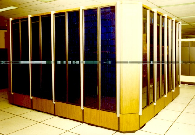
At the same time as the mini-computers were starting to arrive, we had the next generation of large machines show up -- our first generation of commercial machines. Our supercomputer of the day was the Control Data Corporation (CDC) Cyber 7600, which looked like this. It had this really cool wood and blue glass look to it which, looks kind of dated these days, but was really spectacular back then. This was a very fast machine. This system here ran in the 20 to 40 million instruction per second range. Nearly a hundred times faster than the BRLESC-II.
The next stage in the evolution goes back in the mini-computer category. This is a VAX 11/780. These are the machines, 32-bit computers, that started replacing the minis. These are every bit as capable as the super computers we were using just a few years ago. This machine here blows BRLESC-II off the map. This is the sort of thing you would find in every division, in every computer room sprinkled around all over the place. So you see how this technology keeps moving diagonally across this chart.

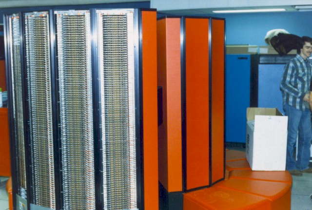
The super computer of the day then was the Denelcor HEP which was
largely
due to the vision of Dr. Eichelberger and this man here,
Clint Frank.
 Here, Clint is
holding one of the processor boards from the Denelcor HEP.
This system was a behemoth, and
took up a lot of floor space, yet still to this
day it is the most
elegantly designed parallel processing system around.
This is the
machine
that all the text books that teach parallel processing refer to.
It was built for BRL
to BRL specs by a little firm in Colorado.
It could deliver 40 MIPS, and had a theoretical peak of almost 40 MFLOPS.
Each of the four Process Execution Modules (PEMs) ran eight
different threads in parallel, context switching between them
on an instruction-by-instruction basis to keep all the pipelines filled.
Here, Clint is
holding one of the processor boards from the Denelcor HEP.
This system was a behemoth, and
took up a lot of floor space, yet still to this
day it is the most
elegantly designed parallel processing system around.
This is the
machine
that all the text books that teach parallel processing refer to.
It was built for BRL
to BRL specs by a little firm in Colorado.
It could deliver 40 MIPS, and had a theoretical peak of almost 40 MFLOPS.
Each of the four Process Execution Modules (PEMs) ran eight
different threads in parallel, context switching between them
on an instruction-by-instruction basis to keep all the pipelines filled.
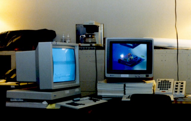
Work stations finally came to life. The Sun-2 computers started showing up, and that changed what was happening at the desk top quite a bit. This is a picture of my desk in 1985. This sets the trend for everything that has followed. It was a Sun-2 workstation here on the left. This was a quarter million instruction per second black and white workstation and a Silicon Graphics 3030 which had real-time, wire-frame rotation. We could do target descriptions very, very rapidly on them. This really set the whole direction for VLD.

At the same time, departmental computers got a whole heck of a lot faster. This is a Gould 9000, it has a dual CPU system delivering ten million instructions per second; a pretty good fraction of what the Cyber 7600 was giving just a few years earlier. Amusingly enough, this machine was created for BRL; Chuck Kennedy and I managed to convince Gould management that it would be very inexpensive to add virtual memory to their speedy Concept 32/87 CPU.
Between BRL and HEL, we bought 14 of these machines at a very low price in the space of about two years. Really goosing up the amount of compute power available locally in the divisions.
In 1986, things go a little further and the Cray XMP shows up. This really blasts us ahead. Here you can see Phil Dykstra helping to unpack this box on the very first week the XMP was being installed. This machine, a super computer of the day, is still running here at BRL today, but its performance is no longer particularly considered in the super computer category.
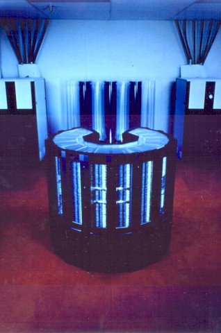
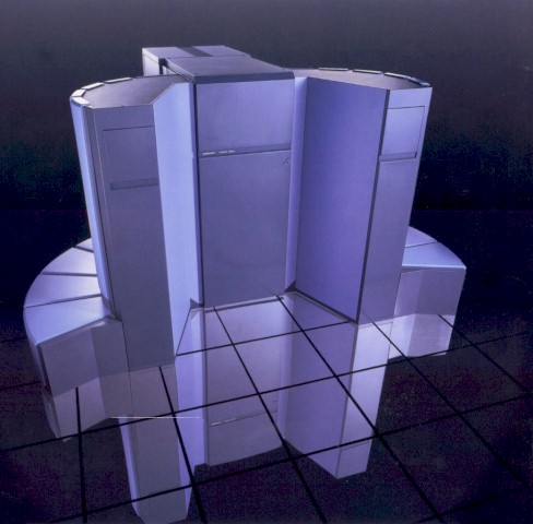
A year later, this machine rolled in. The Cray-2 called "Bob" in honor of Dr. Robert Eichelberger. This machine, at the time, was the fastest machine on the planet, again putting BRL back on the forefront. With an astonishing two gigabytes of main memory, this machine has so much main memory sitting inside this tank that it takes two full hard disk drives just to take a crash dump when the machine goes down. The disk drives only hold one gigabyte (memory was two gigabytes) and these are big quarter million dollar disk drives this thing uses. It is kind of a strange twist where main memory is getting to be bigger than disk drives in some cases.
Just a few years ago the Corps of Engineers finally got a Cray YMP, which we can use over the network. This is what is looks like, if you were to go down there and visit it. So, there has been a tremendous amount of evolution here.
In the mini computer department, SGI predators (which I don't have a picture of), are machines that now rival the performance of the Cray XMP48. They cost about one-quarter million dollars and are turning up all over the place. So you can see with a time lag of about five years what is over here moves over to the center column and what is over here in the center column moves on to the desk top. This is a trend that is just going to keep going.
Now with all this evolution in hardware, what has been happening in software? We made some very good choices back in 1979 and 1980 which have stood us in tremendous good stead. Our first 11/70 ran UNIX and, as part of that plan for the 1980s, we said all the computers at BRL really ought to run UNIX if they can.
Some advantages from this include portable code, and portable scientists. When you replace the hardware instead of going through a massive retraining switching from the BRLESC to the Cyber, from Cyber to the UNIX, it now means just changing from one variant of UNIX to the other. Instead of requiring weeks and weeks to refamiliarize yourself, it is just a matter of a few hours learning this little nit, that little nit, some new performance options. Also, as software developers, you save a lot of time porting software. Most of our software has run across five generations of hardware now with little or no changes. Considering some of our big packages are huge, million-line and above type, software packages developed locally, the portable application software is not to be sneezed at.
This gave us the ubiquitous standardized environment for doing everything; for doing scientific calculations, for doing document processing, for doing E-mail communicating with the outside world. All happening in this one platform. I note, sadly, that a lot of Army facilities, even some parts of ARL, don't even have working e-mail yet. So we managed to knock all this off in the early 1980s and not struggle a lot on the simple things.
There have been a few things that have changed in UNIX over the years and I won't bore you with all the computer science details other than to note that now it is available in almost everything all the way from the MAC-II and the PC up to the Cray-II. UNIX grew to embody network services adding network file systems, remote procedure calls, distributed compilations and all that graphically user interfaces with bit maps especially using MIT's X-window system, parallel processing, virtual memory. The ANSI version of the C programming language was done in large measure by Doug Gwyn here at BRL. He gets a tremendous amount of credit for helping to take the C programming language which UNIX is based on and turning it into a standardized computing language, which is used now the world over.
To make these machines all talk together, we needed to invent some networks. Originally, computing was easy. There were one or two computers and you went to them and did your work there. But when we started having first a dozen and then hundreds of machines around here, computers became much more distributed, and it was not always easy to get your data from the computer on which the data were stored to the one you wanted to use to compute these data on. To solve that problem, we needed to build networks.
It was the campus area net hooking together the buildings and the laboratory that really took the most work. We did some really interesting experiments here in 1980 duplicating what the ARPANET had done using 56 kilobit communication lines and that served us very well all the way up to 1985 when we finally got fiber optics in the ground - a task that took three years from start to finish.
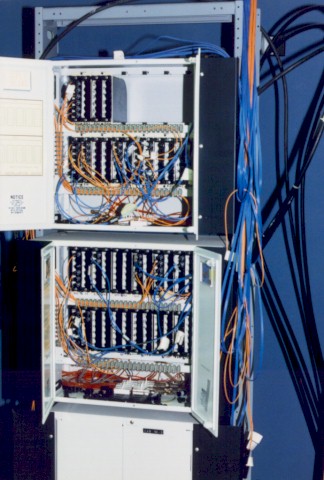 Here is the main hub of the Building 328 fiber optics patchbay.
The photograph is from 1985, it's actually jammed full now. Each
of these colored
ribbons here is a thin piece of glass fiber optic carrying, in some
cases, as
much as 100 megabits of data on it. You can see this is a lot like
the plug
boards of old. You can plug these ultra high bandwidth fiber optics
into these
little bi-conic sockets, screw them down, and make a super high bandwidth
connection from building to building. That spurred the growth
of first ten,
then 80, and now 100 megabits per second communication links between
the
buildings.
Here is the main hub of the Building 328 fiber optics patchbay.
The photograph is from 1985, it's actually jammed full now. Each
of these colored
ribbons here is a thin piece of glass fiber optic carrying, in some
cases, as
much as 100 megabits of data on it. You can see this is a lot like
the plug
boards of old. You can plug these ultra high bandwidth fiber optics
into these
little bi-conic sockets, screw them down, and make a super high bandwidth
connection from building to building. That spurred the growth
of first ten,
then 80, and now 100 megabits per second communication links between
the
buildings.
I also want to note that there was a matching effort replicating all of this network connectivity at the SECRET level. That work started around 1985 and has carried forward as well. So that now in VLD we have secret level communication between buildings 394, 328, and some of the other parts of BRL compound here, with direct connectivity across the wide-area DISNET to many other secret facilities inside the DoD.
These are some historic events in networking. I don't want to bore you with all these, except to note that in history books remote computing was first done around 1965 or so. BRL did it first in 1953 using the then extensive teletype network of Western Union. The ORDVAC computer had the option of reading and writing its output on paper tapes. What people would do is they would send a telex to BRL with the program on paper tape. The people at University of Illinois, National Bureau of Standards, and other institutions would Western Union in one of these paper tapes, the operator at the ORDVAC would tear it off, stick it in the machine, and it would calculate for while, they would tear the paper off the output punch, send it back to Western Union, and zip it across the country - in 1953, network computing.
We spent a lot of time in the early 1980s working on electronic mail and the TCP/IP protocols. It was very gratifying in 1984, all this home brew stuff that we had been fussing around with DARPA became military standard. All the work that we did here wound up embodied in Military Standard 1777 and 1778. This is now the foundation for the communications throughout the world. All the universities everywhere run these communications protocols, and we had a big hand in building that. First super computer on the internet, first classified campus nets are some other firsts that happened here at BRL.
In the software department, BRL invented a whole technology - solid modeling. Dave Rigotti, I think, gets the credit for starting this one in 1958, the year I was born. He was thinking about nuclear problems and stimulated the research that wound up in MAGIC in the SAM-C codes being built about the year 1967. (Editor's comment: While a good deal of inspiration came from the nuclear people, there was also heavy involvement of more conventional ballisticians such as Hoyt and Peterson.) That was the foundation of everything BRL and then AMSAA went off to do looking both at computerized conventional vulnerability and computerized nuclear vulnerability.
The second generation of software was GIFT geometric information from targets and then around 1985 we began a transition to what we now calling BRL-CAD® which is a UNIX based C implementation of this same solid modeling technology. Most of you probably know BRL-CAD® best for MGED its geometry editor program. But it is also LIBRT, the library for ray tracing geometry, and this is a nice object oriented separation of the geometry part which us computer scientists types worry about and the applications part which more physics oriented people might concern themselves with. This allows advances in each of those to be decoupled so that as the geometry stuff gets better the applications automatically benefit, as the applications gets smarter they do not necessarily impact what has to be provided to them on the geometry side.
There is a whole family of codes; RT and LGT, for making nice shaded pictures like this one over here; SQuASH, which you are going to hear about more later on; stochastic high res modeling; SPRAE, you are going to hear about a fantastic piece of work done with the Command Post using this; and MUVES, our brand new modular environment for doing all new vulnerability codes in.
In addition to all this, there are 174 other tools and 14 software libraries which comprise this product called BRL-CAD®. It is supported on ten different kinds of hardware and in use by more than 800 institutions world wide which makes it, I think, one of our premier technology transfer examples as well. This is all stuff that was done first here at BRL. So to show you just a hint of the complexity of all this each of the ovals here is a library, each of the double boxes is a file format, each of the single boxes is an analysis program. I don't expect you to understand all this but to merely use this as a big picture road map of some of the complexity involved in doing all of this CAD work. A tremendous amount of software and a significant amount of design went into that, and a lot of that research continues on to this day with new techniques being added like n-manifold geometry and a lot of sophisticated visualization techniques.
We have ubiquitous unix based computing and printing, we have had it for a long time. I might point out that these slides here are all done on a UNIX based printer. This is really nice being able to just say "print me up an ENIAC" and you get this marvelous viewgraph of an ENIAC. Lee Butler over here gets the credit for acquiring the scanning and printing hardware that made this talk possible.
We have a workstation and a PC for every employee -- more than ten MIPS of CPU power for every employee in VLD. Now I don't say that its evenly distributed, some have a little more, some have a little less. But if you tally it all up, there is a tremendous amount of power here. More than 150 computer systems, Chuck Kennedy might have an even better number, you almost have to track this daily as the trucks keep rolling in with more and more computers. More than 100 gigabytes of on-line storage. This isn't tapes, this isn't stuff found in a closet. This is 100 gigabytes of storage that is running right now that anybody could get access to at 1 or 3 megabytes per second, zoom that data in, and process it. Even taking out target libraries and system overhead and all of that, that is more than 100 megabytes per employee -- an order of magnitude higher than the goal we had set for 1989.
We have separate unclassified and SECRET level networks and while the secret level network does not get everywhere yet (in particular it is not on every desk top) it will be in another couple of years and that is going to really revolutionize the way things are done.
Distributed computing: The file server and compute server that I use now today has the same performance as the Cray XMP. Well, it has a 5 year technology advantage, so that is not as surprising as I made it sound. But it really boggles my mind to think that the computer that we struggled so hard to buy from 1980 to 1985, the Cray, you can now go out and duplicate for one-quarter million dollars!
Sophisticated color scanning, printing, computer generated video tapes (which I do not have time in this talk to show you) -- all this we have now at VLD and use it to great advantage.
A good news chart is shown in Figure 36. Our computing capacity in 1983 was one VAX-11/780 equivalent and was 3,155 times that capacity by 1989. The numbers just keep going up from there. I'll try to show you how price and performance change with time, time is not an axis on here, we have price versus performance and log-log plot you can see super computers lie over in here, the departmental machines lie in the middle, and the workstations tend to lie over here. The dots just keep drifting off. In terms of ray-tracing performance, which is what most of our vulnerability calculations require, here is a plot of relative performance on that problem of the different kinds of machines. You can see right here the Cray XMP and the Silicon Graphics predator. For this particular test, the XMP has very slight edge. But these predators are just riddled throughout the place. They are located all over now. So that everyone has access to their "own" XMP-class machine. And that is how it should be.
I would like to acknowledge a bunch of people for helping me collect the facts I used to prepare this talk. Harold Breaux, Chuck Kennedy, Lee Butler, Phil Dykstra, Bob Reschly, and Bert Meyer all contributed background material that I synthesized together to give you this. Because especially for the first part, I was not around.
That is the end of my presentation. I would actually like to keep going for another hour or more, but you are probably going to throw me out. I am afraid there is no time for questions.
I welcome comments, suggestions, and additional information -- especially URLs or written references to other historic computers. Please feel free to send me E-mail, or FAX me at USA 410-278-5058.
Images of all of the computers mentioned in this talk are available in RGB, GIF, and JPEG format from https://ftp.arl.army.mil as are photo credits and photo captions .